Heard about Excel’s VLOOKUP for quite some times, but still not sure what it does and what it use for. Having help my friend with some files, I learned that Excel can be quite flexible.
My friend are required to prepare a Excel report/form that need to draw data from another sheet, which will shows in a convenient drop down list, after selected, the other respective cell should automatically filled.
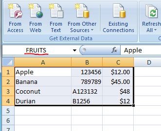
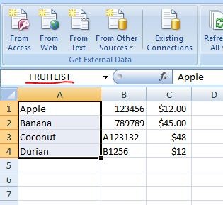
To start, we need to create a data list in a sheet, for example sake, I used fruits as the list, with some sample fruit’s code and price for each. Now I need to prepare the name for future use, select all the fruits name, and key in the name ‘FRUITLIST’ as the name, and hit enter.
The fruit list is for the drop down list data source, now we need to create a list for the other cell to retrieve data when the fruit’s name are selected.

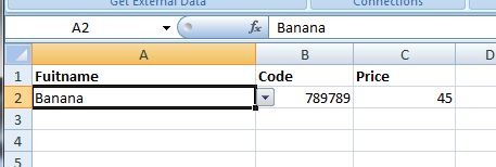
Now, on my second sheet, on the cell that wanted to serve as drop down list, select Data from the menu, and then Data Validation. On the Data Validation window, choose List for the Allow, and =FRUITLIST as the Source, and click OK. Now the cell got a little arrow on the right hand side, click on it should show the list of the fruits from sheet 1.
On the cell that we wanted to show the code, we key in the formulae =IF(A2=””,””,VLOOKUP(A2,FRUITS,2)), where A2 is the cell where we created it as drop down list, first, we use the IF statement to check for A2 value, means if we did not choose anything from the list, this cell will be empty, else, we use the VLOOKUP to grab data, first parameter A2 is what we want to lookup, second parameter, FRUITS is where we want to lookup from, and the 2 is which column (it is the column for the FRUITS, but not sheet1).
Now when we choose the fruits from the list, the Code and the Price (will need to use the same formulae used on Code, but with different column) will be auto populated.

